Test cases
Shock tube
Shock tube test case is comprised of a tube of unit length containing initially two gases separated by an imaginary membrane at x = 0.
Mesh properties
Mesh is comprised of 100 cells.
Initial condition
Flow is initizalized by reading flow_init.ini.
Variable |
Left |
Right |
|---|---|---|
Density |
1.0 |
0.125 |
Pressure |
1.0 |
0.1 |
Velocity |
0.0 |
0.0 |
Flow type |
Unsteady |
Riemannsolver |
Roe |
Temporal discretization |
Runge-Kutta (4-stage) |
Scheme |
MUSCL |
Limiter |
Venkatakrishnan (K = 0.3), Barth-Jespersen |
Time step |
1e-3 |
Number of time steps |
200 |
Boundary condition
Flow in the tube is made one-dimensional by imposing empty boundary conditions in peripheral surfaces of the tube. At caps of the tube, dirichlet boundary condition is imposed.
Results
Following results correspond to \(t = 0.2\) seconds.
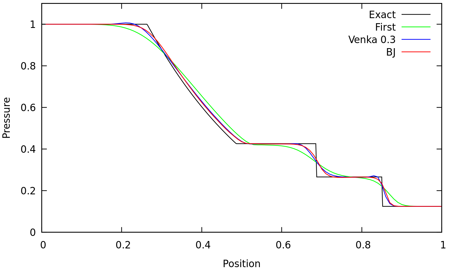
Remarks
Second order spatially-accurate results are better than first order one.
A limiter is required otherwise the code blows up if only gradient is used for flux reconstruction at cell-faces.
Venkatakrishnan limiter with coefficient of \(K=0.3\) is not TVD, hence, overshoots are observed near discontinuities.
Steady transonic airfoil
A single unstructured mesh is used to solve the Euler equations at transonic air speed to steady state. Flow and solver properties are shown in the following tables. The mesh is rotated \(1.25^\circ\) clock-wise, therefore, the freestream x-velocity has no angle of attack. Freestream pressure and density are adjusted such that sound speed is unity and freestream velocity is identical to Mach number.
Mach |
0.8 |
Angle of attack |
\(1.25^\circ\) |
Freestream pressure |
1 / 1.4 |
Freestream density |
1 |
Ratio of specific heats |
1.4 |
Reference area |
1 |
Flow type |
Steady |
Riemann solver |
Roe |
Temporal discretization |
Backward Euler |
Scheme |
MUSCL |
Gradient computation |
Least-squares |
Limiter |
Venkatakrishnan (K = 0.3) |
CFL |
10 |
Settings are read from settings.ini.
Mesh properties
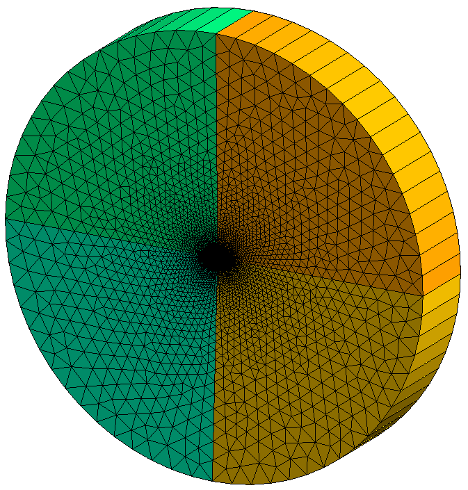
Following figures shows the unstructured mesh used for solving transonic airfoil test case.
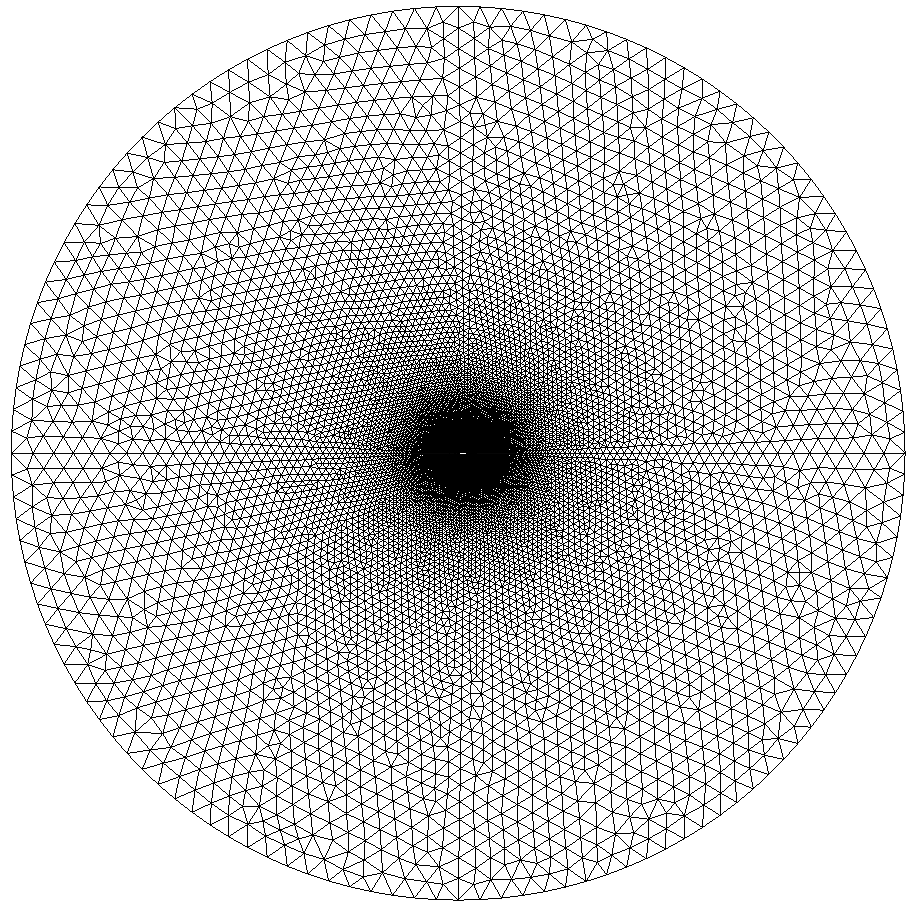
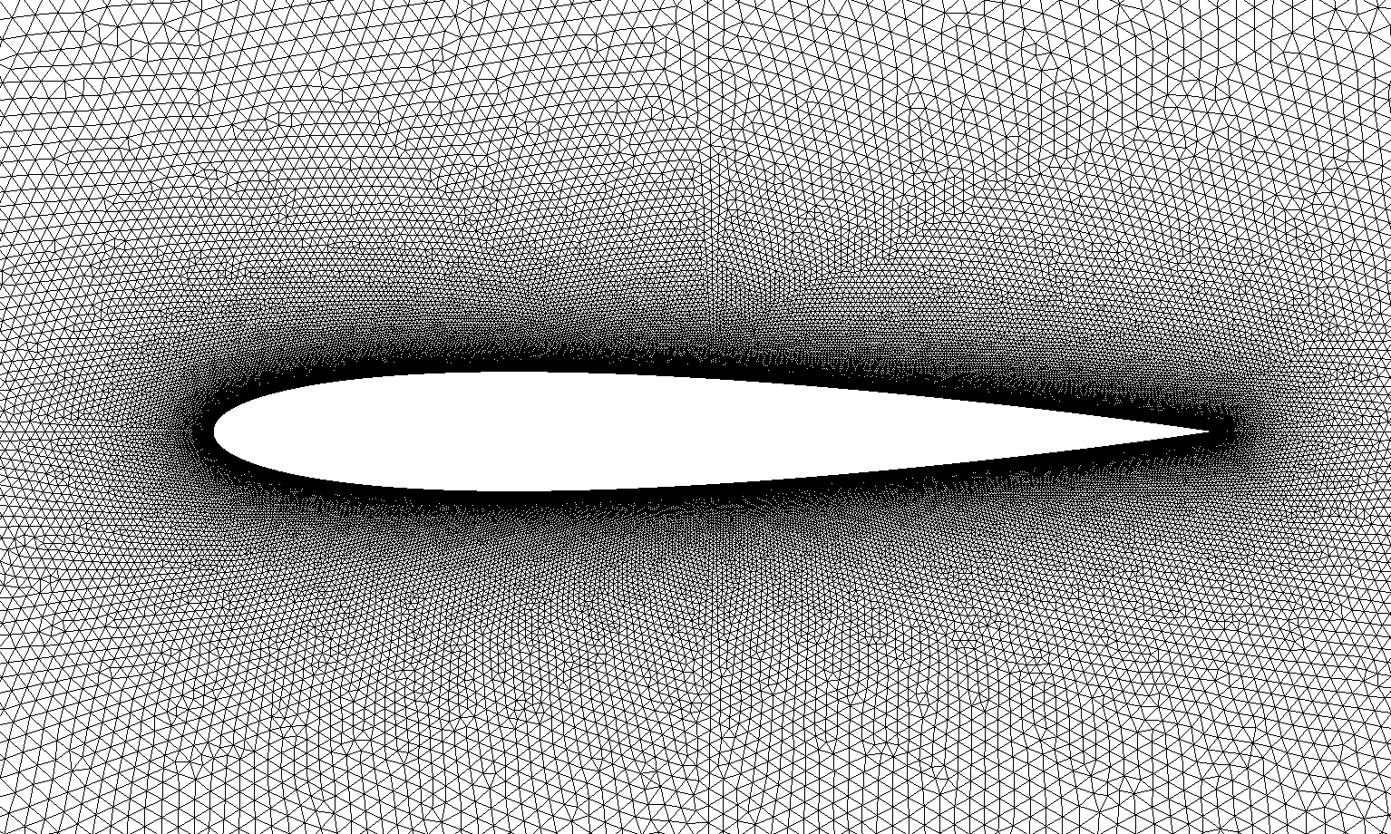

Cell size is the finest near the airfoil and grows proportional to distance from the airfoil surface. Cell size is controlled with combination of Field in NACA0012_O.geo as shown below.:
lc = 1;
Field[1] = Distance;
Field[1].FacesList = {wallbc[]};
Field[1].NNodesByEdge = 100;
Field[2] = MathEval;
Field[2].F = Sprintf("F1/20 + %g", lc / 1000);
Background Field = 2;
According to the snippet above, cell size is set with equation distance/20 + 1/1000. I don’t know how cell size is related to cell volume in Gmsh. There 137228 cells with shape of triangular prism in the unstructured mesh. The reason of having three-dimensional (3D) cells in a two dimensional(2D) problem is because Tailor always works in 3D space similar to OpenFOAM. This kind of problems are called 2.5-dimensional. The 3D mesh is obtained by extruding the 2D mesh by one layer.
Since there 32 processors, initially the mesh is also partitioned into 32 partitions.
gmsh NACA0012_O.geo -3 -oneFilePerPart -part 32 -format msh2
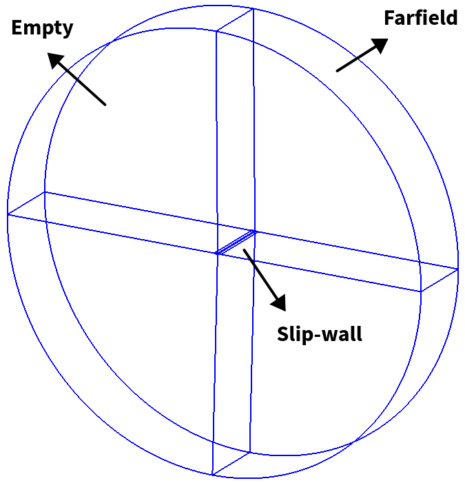
Boundary conditions
Boundary conditions on the airfoil and in outer boundary are slip-wall and Riemann, respectively. Riemann boundary condition is based on Riemann invariant equations. Empty boundary conditions are used in z-normal direction. Initially flow is set to freestream values everywhere in the domain.
Job submission
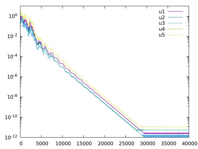
The code works even when CFL is greater than 10 however, residuals do not converge below 1e-2 in that case. The script below is the SLURM script used to submit a job to the cluster.
#!/bin/bash
#SBATCH -p short
#SBATCH --ntasks=32
#SBATCH --hint=nomultithread
#SBATCH -t 00-04:00:00
#SBATCH --output=slurm-%j.out
#SBATCH --error=slurm-%j.err
mpirun --tag-output --report-bindings /usr/bin/time -f '%e %S %U %P %M' -o "timing.dat" --append ./out
Results
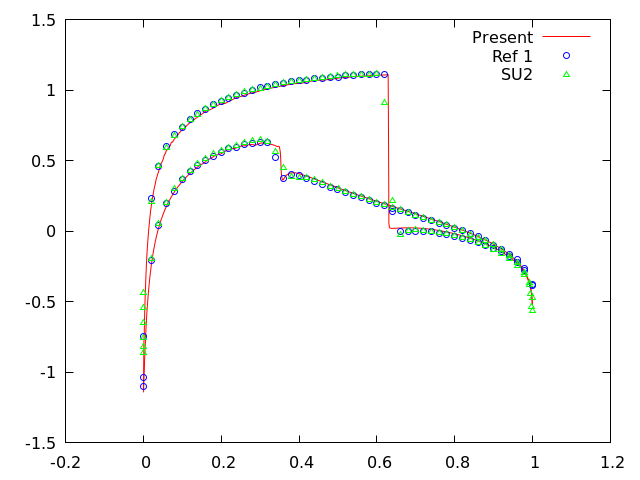
Figure below shows pressure coefficients at the airfoil surface and convergence history.
Remarks
Compared to other references, finer mesh is needed to accurately solve pressure and force coefficients.
There is practically no difference between results of first and second order spatial accuracy. This may be due to steady state solution.
It is useful to have raw pressure coefficient data to compare results, especially when data for upper and lower surfaces are provided separately. This saves time by avoiding plot digitizing. Here are pressure coefficient data for upper_pc.dat and lower_pc.dat airfoil surfaces.
References
Reference 1: Manzano, Luis, Jason Lassaline, and David Zingg. “A Newton-Krylov algorithm for the Euler equations using unstructured grids.” 41st Aerospace Sciences Meeting and Exhibit. 2003.
Reference 2: https://su2code.github.io/tutorials/Inviscid_2D_Unconstrained_NACA0012/
Pitching airfoil
A NACA 0012 airfoil undergoes a forced harmonic oscillation while moving against a free-stream with Mach number of \(M=0.755\). This problem can also be solved as static mesh problem by fluctuating the free-stream velocity. The mesh used in steady transonic airfoil problem is also used here except that the initially the airfoil mesh is rotated \(2.51^\circ\) instead of \(1.25^\circ\).
Mesh oscillates with instantaneous angle
where, \(\alpha_{mean}\), \(\alpha_{amp}\), \(t\) is the mean, amplitude and time, respectively. \(\alpha_{\omega}\) is the angular frequency found from the reduced frequency
where, \(c\) and \(u_\infty\) are the chord length and free-stream velocity which is the same as Mach number since free-stream pressure and density are adjusted to make speed of sound unity. Table below shows the parameters used to calculate the instantaneous angle of attack.
Mean pitch angle |
\(\alpha_{mean}\) |
\(0.016^\circ\) |
Pitch amplitude |
\(\alpha_{amp}\) |
\(2.51^\circ\) |
Reduced frequency |
\(k\) |
0.0814 |
Chord length |
c |
1 |
Mach |
M |
0.755 |
Results
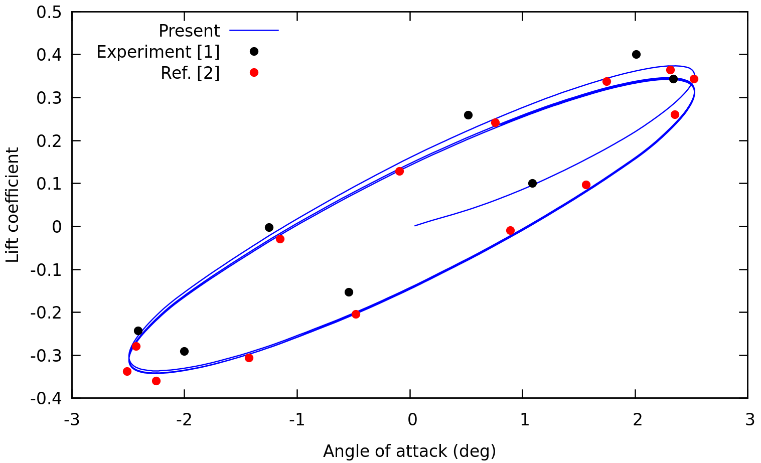
Figure below shows the lift hysteresis. There is a good agreement with the another numerical method. The reason of discrepancy from the experimental lift is due to absence of viscosity in the numerical solution.
References
Reference 1: Landon, R.H., “NACA 0012 Oscillatory and Transient Pitching,” Data Set 3, Compendium of Unsteady Aerodynamic Measurements,” AGARD Report 702, August 1982.
Reference 2: Venkatakrishnan, V., and D. J. Mavriplis. “Implicit method for the computation of unsteady flows on unstructured grids.” Journal of Computational Physics 127.2 (1996): 380-397.