Test cases

Shock tube

Shock tube test case is comprised of a tube containing initially two gases separated by an imaginary membrane at x = 0.

Initial condition

Flow is initizalized by reading flow_init.ini.

Initial profile

Variable	Left	Right
Density	1.0	0.125
Pressure	1.0	0.1
Velocity	0.0	0.0

Solver parameters

Flow type	Steady
Riemannsolver	HLLC
Temporal discretization	Runge-Kutta (4-stage)
Limiter	Venkatakrishnan (K = 0.3)
CFL	10

Boundary condition

Flow in the tube is made one-dimensional by imposing empty boundary conditions in peripheral surfaces of the tube. At caps of the tube, dirichlet boundary condition is imposed.

Results

Steady transonic airfoil

A single unstructured mesh is used to solve the Euler equations at transonic air speed to steady state. Flow and solver properties are shown in the following tables.

Flow properties

Mach	0.8
Angle of attack	\(1.25^\circ\)
Freestream pressure	1 / 1.4
Freestream density	1
Ratio of specific heats	1.4

Solver parameters

Flow type	Steady
Riemann solver	Roe
Temporal discretization	Backward Euler
Limiter	Venkatakrishnan (K = 0.3)
CFL	10

Settings are read from settings.ini.

Mesh properties

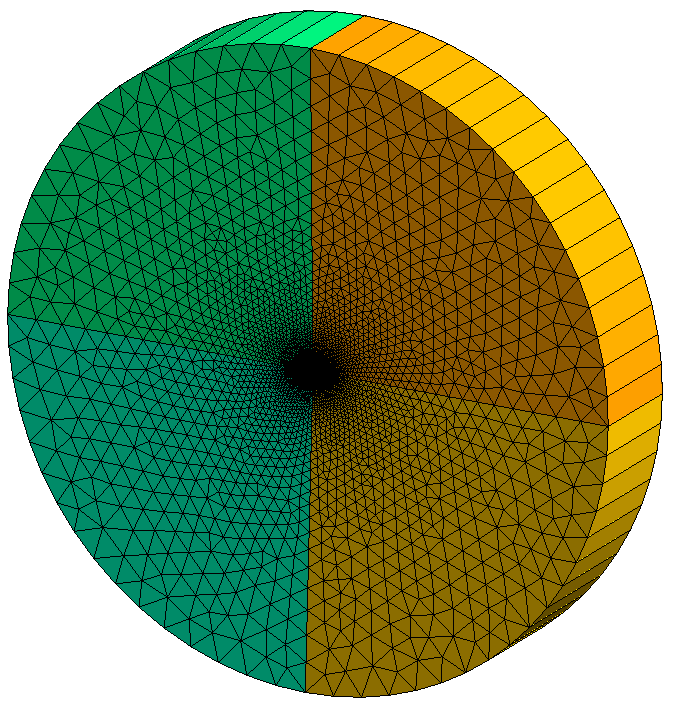
Following figures shows the unstructured mesh used for solving transonic airfoil test case.

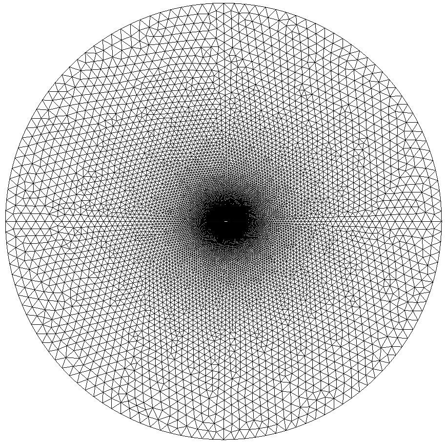
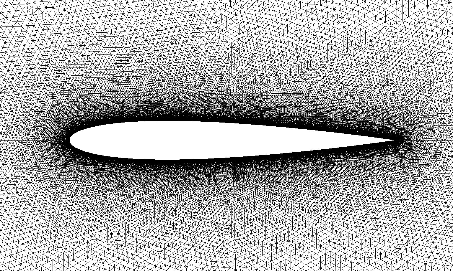
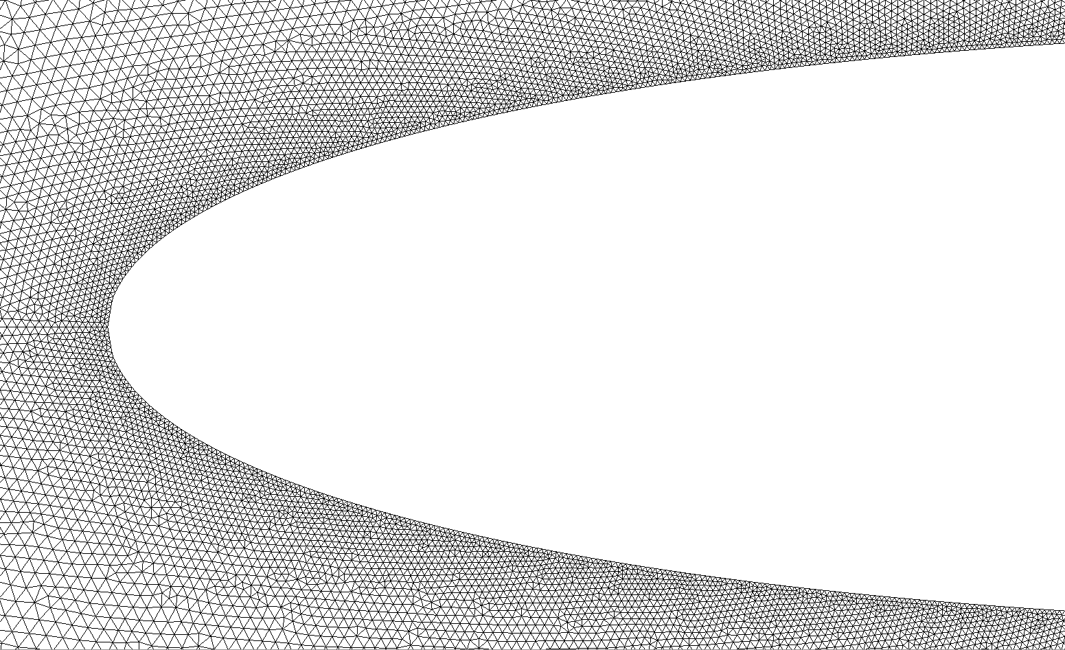
Cell size is the finest near the airfoil and grows proportional to distance from the airfoil surface. Cell size is controlled with combination of Field in NACA0012_O.geo as shown below.:

lc = 1;
Field[1] = Distance;
Field[1].FacesList = {wallbc[]};
Field[1].NNodesByEdge = 100;
Field[2] = MathEval;
Field[2].F = Sprintf("F1/20 + %g", lc / 1000);
Background Field = 2;

According to the snippet above, cell size is set with equation distance/20 + 1/1000. I don’t know how cell size is related to cell volume in Gmsh. There 137228 cells with shape of triangular prism in the unstructured mesh. The reason of having three-dimensional (3D) cells in a two dimensional(2D) problem is because Tailor always works in 3D space similar to OpenFOAM. This kind of problems are called 2.5-dimensional. The 3D mesh is obtained by extruding the 2D mesh by one layer.

Since there 32 processors, initially the mesh is also partitioned into 32 partitions.

gmsh NACA0012_O.geo -3 -oneFilePerPart -part 32 -format msh2

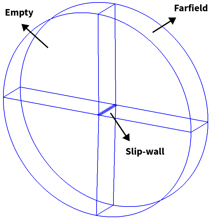
Boundary conditions

Boundary conditions on the airfoil and in outer boundary are slip-wall and Riemann, respectively. Riemann boundary condition is based on Riemann invariant equations. Empty boundary conditions are used in z-normal direction. Initially flow is set to freestream values everywhere in the domain.

Job submission

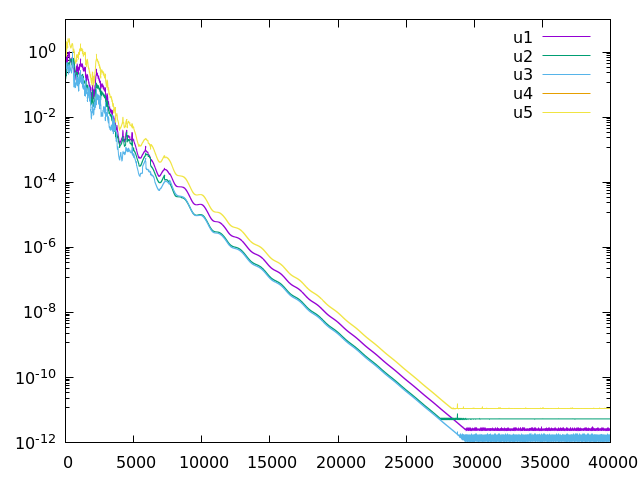
The code works even when CFL is greater than 10 however, residuals do not converge below 1e-2 in that case. The script below is the SLURM script used to submit a job to the cluster.

#!/bin/bash
#SBATCH -p short
#SBATCH --ntasks=32
#SBATCH --hint=nomultithread
#SBATCH -t 00-04:00:00
#SBATCH --output=slurm-%j.out
#SBATCH --error=slurm-%j.err
mpirun --tag-output --report-bindings /usr/bin/time -f '%e %S %U %P %M' -o "timing.dat" --append ./out

Results

Figure below shows pressure coefficients at the airfoil surface and convergence history.

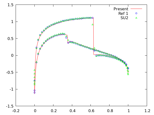
It is useful to have raw pressure coefficient data to compare results, especially when data for upper and lower surfaces are provided separately. This saves time by avoiding plot digitizing. Here are pressure coefficient data for upper_pc.dat and lower_pc.dat airfoil surfaces.

Reference 1: Manzano, Luis, Jason Lassaline, and David Zingg. “A Newton-Krylov algorithm for the Euler equations using unstructured grids.” 41st Aerospace Sciences Meeting and Exhibit. 2003. Reference 2: https://su2code.github.io/tutorials/Inviscid_2D_Unconstrained_NACA0012/

Oscillating airfoil